4. Analysis
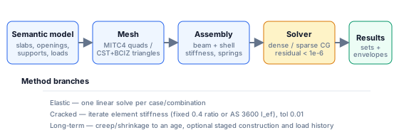
The analysis pipeline is: semantic model → generated mesh → assembled finite
element model → solve → results. Everything in this chapter happens on the
Go server; the browser sends the model and receives results.
4.1 The three analysis methods
The Run analysis modal offers one method at a time, each a superset of the
previous:
| Method | What it solves | Use it for |
|---|---|---|
| Elastic | One linear-elastic solve | Supports, load distribution, most ultimate-strength design moments, reactions |
| Cracked | Iterates element stiffness down where tension exceeds cracking | Realistic deflections and moment redistribution at service load |
| Long-term | Time-stepped creep + shrinkage deflection to an age (optionally staged) | Long-term deflections, deflection-history checks |
Each method can run several load cases/combinations in one pass; every solved
item becomes a result set, and envelopes are built automatically.
Orthogonal to the method, no-tension soil (a soil zone with Compression
only ticked) wraps any run in a contact loop: solve, lift off every
compression-only spring whose node rose, repeat until the contact state
settles (max 20 passes, usually 2–4). Combinations with no-tension soil solve
directly rather than by superposition. See
§7.1.
4.2 Mesh generation (MESH)
Before running, the model must be meshed. MESH opens Mesh Generation:
| Field | Default | Options |
|---|---|---|
| Mesh Type | Quad (structured) | Quad / Triangle |
| Element Size (m) | average slab size or 1.0 | ≥ 0.1 |
Generate Mesh writes the mesh type and each slab's mesh size, then meshes.
Clear Mesh discards it. The meshing rules and element formulations are in
§2.18.
Normally you do not need this dialog: Run Analysis regenerates the mesh
automatically, and the slab tool's own Mesh size field controls refinement.
4.3 Validate (CHK)
CHK runs ValidateAll = semantic validation + mesh build + mesh checks
(duplicate nodes/elements, degenerate elements, disconnected components,
stray restraints). See §2.17 for the
full message list. Validation is the cheapest way to catch model problems;
the run refuses models with errors.
4.4 The Run analysis modal
Toolbar: ▶ Run Analysis. The modal has a live This run summary and
status banner; Close dismisses it, Run Analysis starts the run
(button changes to Running… and disables). The modal cannot be closed
during a run, and there is no abort button - navigating away cancels the
request (the server logs it as client closed the request).
Step 1 - Method
Tabs: Elastic, Cracked, Long-term.
Elastic
No options. The default and fastest method. One linear solve per selected load
item; combination superposition is used where possible.
Cracked - fields
| Field | Unit | Default | Range | Notes |
|---|---|---|---|---|
| Nonlinear cracked | – | selected | – | radio; the method requires it |
| Cracked E/Ec | ratio | 0.4 | 0.01–1, step 0.01 | fixed stiffness reduction for cracked elements |
| Max iterations | – | 20 | 2–100 | iteration cap |
| ρ-dependent stiffness (AS 3600 I_ef) | – | off | – | computes I_ef per element from the provided steel |
| fy | MPa | 500 | 100–2000 | ρ-dependent mode |
| Cover | mm | 30 | 10–100 | ρ-dependent mode |
Fixed-ratio mode is a simple secant method: elements whose tensile demand
exceeds the concrete tensile strength progressively relax toward E/Ec = 0.4
(default), uncracked elements return to 1.0, with under-relaxation 0.6 and a
0.01 relative convergence tolerance. It answers "how much softer is this slab
once it cracks" without needing reinforcement data.
ρ-dependent mode computes a real cracked section per element:
n   = Es / Ec
Icr from the transformed cracked section (As, d, b = 1000 mm)
Mcr = fct × t²/6 × 1000              [kN·m/m]
Ief = Icr / [1 − (1 − Icr/Ig)(Mcr/Ms)²]     (AS 3600 Cl 8.5.3.2 / ACI Eq. 24.2.3.5b)
Ief ≤ 0.6·Ig when pt = As/d < 0.005          (AS 3600 cap)
ratio = Ief / Ig
When strip reinforcement is available the per-element steel is taken from the
strip; otherwise the entered Ast/Asc values apply. Concrete tensile strength:
0.6√f′c (AS 3600/CSA), 0.62√f′c (ACI), 0.30·f′c^(2/3) (EC2/default).
Cracked runs report iterations, converged flag, cracked element count and the
residual history (plotted in Charts → Convergence). If iteration stalls:
reduce the ratio, raise Max iterations, or use the fixed-ratio mode.
Long-term - fields
| Field | Unit | Default | Range | Notes |
|---|---|---|---|---|
| Long-term deflection | – | off | – | enables the time-dependent model |
| Long-term deflection code | – | AS 3600 - φcc + kcs | AS 3600 / ACI 318 | method for creep + shrinkage |
| Duration | days | 3650 (10 yr) | 1–100 000 | analysis horizon |
| Bottom steel Ast | mm²/m | 500 | step 25 | midspan, per metre width |
| Top steel Asc | mm²/m | 500 | step 25 | midspan, per metre |
| Effective depth d | mm | 150 | 40–1000 | ACI path (and fallback) |
| Concrete grade | – | active code grades, default 32 MPa | – | AS 3600 path |
| Age at loading τ | days | 28 | 7–3650 | AS 3600 path |
| Member thickness t_h | mm | 200 | 50–1000 | AS 3600 drying path |
| Environment k4 | – | Interior 0.65 | Arid 0.70 / Interior 0.65 / Temperate 0.60 / Coastal 0.50 | AS 3600 Table 3.1.8.3 |
| Strength k5 | – | 1.0 | 0.6–1.0, step 0.05 | AS 3600 |
| Override φcc | – | off, value 1.91 | 0–10 | hold the ultimate φcc |
| Override kcs | – | off, value 0.80 | 0–4 | hold the ultimate kcs |
| Staged construction | – | off | – | reveals the stage editor (§4.5) |
Read-outs show the computed φcc = …, kcs = …, and for ACI
ρ′ = … → λΔ = …. Σ Calculate φcc opens the Creep Factor Calculator
(f′c 32, τ 28 d, time 10 950 d default, t_h 200 mm, k4 0.65, k5 1.0) with a
Use this value button that writes φcc into the override.
AS 3600 model (Cl 3.1.8.3 / 8.5.3.2):
growth(t) = 1 + φcc(t) + kcs × k2(t)

k2  = t^0.8 / (t^0.8 + 0.15·t_h)          (≤ 1; t in days, t_h in mm)
k3  = 1.28 τ^(−0.118)
φcc.b from Table 3.1.8.2:
      f'c  20    25    32    40    50    65    80    100
      φcc.b 5.2   4.2   3.4   2.8   2.4   2.0   1.7   1.5
φcc = k2 · k3 · k4 · k5 · φcc.b
kcs = max(0.8, 2 − 1.2·Asc/Ast)  (≤ 2);   Ast = 0 → 0.8
The solver applies the growth to the sustained load effects only; transient
cases contribute their instantaneous deflection. The result set gains a
time-history curve you can scrub with the Time slider, and the Deflection
selector offers Short-term (instantaneous), Sustained (creep, no
shrinkage) and Long-term (creep + shrinkage).
ACI 318 model (Table 24.2.4.1.3):
λΔ = ξ(t) / (1 + 50 ρ′),     ρ′ = Asc / (1000·d)   [d in mm]
ξ(t):  < 3 mo   m/3
       3–6 mo   1 + 0.2(m−3)/3
       6–12 mo  1.2 + 0.2(m−6)/6
       1–5 yr   1.4 + 0.6(m−12)/48
       ≥ 5 yr   2.0
shrinkage is folded into λΔ
Stage ages are measured from the previous stage; the horizon defaults to
2 000 days if the entered duration is not positive, clamped 1–100 000, and the
deflection-time curve is sampled at 32 points with factor(0) = 1.
4.5 Staged construction
Tick Staged construction to reveal the Stages editor. Default stages
when first opened:
| # | Name | Age (days) | Cases |
|---|---|---|---|
| 1 | Self weight + construction | 0 | the first self-weight case |
| 2 | Superimposed + live | 30 | all remaining cases |
Each stage card has: name, age (days after the previous stage), checkboxes
for cases (SW marked amber) and combinations, and a remove ×. + Add stage
adds a stage at age 30 with all cases selected. Stages with no load items are
dropped before the run; a stage with no explicit ids acts as a catch-all.
Semantics:
- A staged run evaluates the structure stage by stage, accumulating deflection
history over time with the creep model applied from each load's application
age. - Per-stage factors come from the selected combos; self weight is included when
any contributing case carries the SW flag. - The run produces one result set labelled Staged construction, and
the time-dependent curve is labelled Load History; the time slider then
walks the construction history. - If the model needs cracking as well, the cracked iteration runs inside each
stage; failure to converge there aborts with
stage N: cracked iteration did not converge.
Staged construction is the right tool for staged pours, backpropping questions
and "when do I strike the props" studies - not for ordinary single-stage
floors.
4.6 Step 2 - Loads
Described in §3.7. Points to
remember:
- every case and combination is selected by default;
- the
Sustained / Short-termselector per row feeds the long-term run; - Envelope: max and Envelope: min appear once two or more items are
solved; - a run with many combinations means many solves and a longer wait.
4.7 Running and reading the summary
After Run Analysis the status banner shows progress
(Solving <label> (i/n)…), then Analysis complete. The summary rows:
| Row | Meaning |
|---|---|
| Nodes / Elements | mesh size; elements shown as N shells, M beams |
| Max displacement | largest nodal displacement (m in model units, displayed in deflection units) |
| Max stress | peak element stress; for slab models this row shows the equilibrium residual instead |
| Solver | displayed luma_fem; hover for the exact method (local-3d-fem-sparse-cg, -combo, -dense-retry…, etc.) |
| Iterations / ΣRz | cracked iterations when nonlinear; otherwise the ground reaction total from equilibrium |
| Cracked elements | n of N cracked in the final iteration |
| Long-term max δ | last point of the time curve when long-term is on |
Reliability behaviour on the server:
| Situation | Response |
|---|---|
| A solve per user already running | 429 concurrent_solve - "Another analysis is already running…"; the client retries automatically |
| Global solver slots busy | 503 solver_busy - "Solver busy" |
| Rate limit | 429 rate_limited with Retry-After; the client retries |
| Floating island found before solving | 422 with the island report (fail fast) |
| Singular stiffness matrix | 422 with a stability hint |
| Client navigated away | request cancelled (client closed the request) |
The client retries 429s up to 6 times (2–10 s waits) and concurrent-solve
collisions up to 10 times (5–15 s waits). You can close the modal only by
finishing the run.
4.8 Solver internals you may need
Element formulations
| Element | Nodes | Formulation |
|---|---|---|
| Quad shell | 4 | MITC4 (membrane + bending + transverse shear), 6 DOF/node |
| Triangle shell | 3 | CST membrane + BCIZ thin-plate bending + drilling stabilization |
| Beam/column/pile link | 2 | 3D Euler-Bernoulli/Timoshenko beam with axial, Iy, Iz, J and optional end releases |
Solution
- Dense direct solver up to ~2,896 free DOF (64 MiB), accepted only if the
true relative residual ≤ 1e-6; otherwise the model is reported singular with
the actual residual. - Larger models use Jacobi/Block-Schwarz or incomplete-Cholesky preconditioned
CG, falling back to BiCGSTAB, with a dense retry up to ~8,191 DOF. - Targets: relative residual 1e-10; practical acceptance 1e-8 relative /
1e-6 absolute after 200 iterations; a verified true residual ≤ 1e-6 accepts
the result. The iteration cap is8nclamped to [200, 20 000]. - Cracked iterations use a loose intermediate tolerance (1e-4); the reported
result always comes from a full-accuracy solve.
Restraints and stability
- In 3D, suspended models without enough column restraint fix the in-plane
translations (and drilling rotations where plates exist). Slab-on-ground and
pile models instead get only the minimum planar pins, so the slab can deform
in-plane and edge walls lean outward with the slab; pile groups with lateral
stiffness restrain in-plane motion themselves, and only a single
laterally-stiff pile gets the pins (one point cannot restrain in-plane
rotation). - Support types: fixed (all 6 DOF), pinned, rollers and per-axis pins; each DOF
can carry a prescribed displacement. - Springs contribute directly to the diagonal:
Kx, Ky, Kz, Krx, Kry, Krz.
A pile head's rotational spring falls back to the plainKrvalue.
Equilibrium report
For every solve the server computes the applied and reaction resultants about
the origin, the imbalance and the maximum free-DOF residual. The ground-total
shown in the reactions table combines restrained-node reactions with mesh
spring forces (Σ(−kz·uz)). This is the number to compare against hand
calculations: applied ΣFz should equal ground reaction with opposite sign.
4.9 Analysis quality checklist
Before trusting a run:
- Validation clean - CHK reports no errors (warnings checked).
- Equilibrium closes - applied ΣFz ≈ ΣRz (within ~0.1 % for normal
models). - Envelope sanity - ULS moments ≥ SLS moments; min-deflection envelope
is not absurdly larger than a single case. - Mesh sensitivity - halve the mesh size once; peak moments should change
by a few per cent, punching shear by a little more. If not, refine further. - Cracking - cracked deflection should exceed elastic; the cracked
element count should be plausible (tension zones, not the whole slab). - Long-term factor - the growth factor is realistic for the age and
environment (e.g. AS 3600 interior 10-year φcc ≈ 2–3, kcs ≈ 0.8–1.2).
4.10 Troubleshooting
| Message / symptom | Likely cause | Action |
|---|---|---|
reduced system is singular (the model wrings work through a mechanism) |
insufficient lateral restraint / isolated node | add or fix supports; the 422 message names a hint |
singular stiffness matrix: N free DOF(s) have zero diagonal stiffness… |
unrestrained node, degenerate element | run CHK; fix the listed node |
generated mesh has N nodes, above the 5000-node build limit |
mesh too fine | raise the slab Mesh size |
mesh has N disconnected components… |
slabs not touching, wall/column gap | snap edges, add connecting support |
point load N does not lie on the generated slab/column mesh |
point load floating | move it onto a slab, re-mesh |
time options: unknown long-term code … |
internal payload error | reselect the code in the modal |
stage N: cracked iteration did not converge |
stiff cracked loop in a stage | raise iterations, relax ratio, simplify stages |
| Analysis takes very long | many selected combinations, large model | select only the needed cases/combos |
→ Next: Chapter 5 - Results