1. Introduction
Luma is a browser-based finite-element program for the analysis and design of
reinforced-concrete slab systems: suspended flat plates and beams-on-columns,
ground-bearing mats on Winkler soil, pile-supported rafts, slab steps, walls
and edge beams. The model is built as a semantic floor model (slabs,
openings, supports, soil and loads) rather than as raw nodes and elements; the
program generates the mesh, assembles a shell/beam finite-element model, solves
it on the Go server, and renders the results in 3D in the browser.
This chapter covers what the program does, its architecture in enough detail to
use it correctly, the units/sign conventions used throughout the manual, the
user interface, the solver limits, and the shortcuts.
1.1 What the program does
| Capability | Detail |
|---|---|
| Analysis | Linear-elastic static FEA of slabs, plates, walls, beams and columns |
| Nonlinear cracking | Iterative cracked-stiffness analysis with fixed E/Ec ratio or AS 3600 ρ-dependent I_ef |
| Time-dependent deflections | Creep and shrinkage deflection vs time - AS 3600 (φcc + kcs) or ACI 318 (λΔ) |
| Staged construction | Multi-stage loading with different ages per stage and a per-stage deflection history |
| Design codes | EN 1992-1-1 (EC2), AS 3600-2018, ACI 318-19, CSA A23.3 |
| Design output | Required steel maps (B1/B2/T1/T2), strip design and sizing, punching utilisation, crack width, steel stress, deflection checks, bar marking plans |
| Supports | Columns (stiff stubs), point supports, piles (axial/lateral springs, layered shaft springs), walls/line supports, soil zones (distributed vertical springs) |
| Loads | Point loads (forces and moments), line loads (UDL), area pressures, wall top line loads, self weight; load cases and factored combinations, envelopes |
| Results | Deflection, moment, stress, strain, bearing, steel, punching, reactions, column/beam/pile/wall diagrams, time-history curves, compare view |
| Files | JSON project files, verification benchmark downloads, punching report (print/PDF) |
Three model modes
Every floor model is in exactly one mode, chosen automatically by what you
draw (FloorModel.mode):
| Mode | Created when | Supports the model |
|---|---|---|
suspended (default) |
columns/walls provided | Columns, point supports, walls, beams |
slab_on_ground |
a soil zone is drawn | Distributed Winkler springs Kz = k × tributary area |
pile_supported |
a pile is placed | Pile head springs and optional layered shaft springs |
Deleting the last pile returns the model to slab_on_ground (if soil zones
exist) or suspended. Soil and pile modes are not combined - a mat-on-piles
model is modelled as pile_supported, optionally with a soil zone for bearing
display; the piles are the actual support.
Analysis chain
semantic floor model  →  mesh generation (Go)  →  FE assembly & solve (Go)  →  results (browser)
   slabs, loads,           MITC4 quads /            dense or sparse CG,          contours, diagrams,
   supports, soils         CST+BCIZ triangles        cracked/long-term loops     tables, reports
The mesh and solve run on the server (/api/projects/:id/analysis-model then
/api/projects/:id/solve); the browser keeps the semantic model, renders
results and performs the reinforcement design arithmetic (flexure, shear,
cracking, punching).
1.2 Model size and solver limits
The solver is sized for typical floor-by-floor design work, not for very large
global models. Limits are enforced with clear messages:
| Quantity | Limit | Where enforced |
|---|---|---|
| Mesh nodes (build limit) | 5,000 | mesh generator, before assembly |
| Nodes (solve request) | 5,000 | solver request validation |
| Elements | 10,000 | solver request validation |
| Supports | 5,000 | solver request validation |
| Springs | 5,000 | solver request validation |
| Loads (all types combined) | 50,000 | solver request validation |
| Element node references | 32 | solver request validation |
| Concurrent solves per user | 1 | server (429 concurrent_solve) |
| Concurrent solves overall | 2 | server (503 solver_busy) |
| Solve rate | 60/min, burst 15 | server (429 rate_limited) |
| Write budget per solve | 30 min | server |
A mesh is rejected during generation if a single slab projects more than 5,000
nodes, or if the total exceeds it:
slab "S1": mesh size 0.25 projects 6120 nodes, above the 5000-node build limit - use a larger mesh size
Practical guidance:
- 0.5–1.0 m mesh is usual for a flat plate; use 0.25–0.5 m near punching
columns only if you accept the node budget. - An 8 × 8 m bay at 1.0 m gives ~81 nodes and 64 quads; a 30 × 30 m floor at
1.0 m gives ~961 nodes and 900 quads. The limit is reached at roughly a
60 × 80 m floor at 1.0 m mesh - split very large floor plans into separate
projects or coarsen away from the region of interest. - Dense direct solution is used up to ~2,900 free DOF. Larger models switch to
a sparse preconditioned CG/BiCGSTAB solver automatically; both are reported
asluma_femin the results summary (hover the row for the exact method).
1.3 Axes, signs and units
Axes
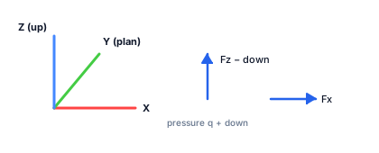
- X and Y are the plan axes. X runs to the right, Y runs "up the page" in
plan. - Z is vertical and positive upwards. Slab elevations, pile head/tip
elevations, wall heights and deflections all use Z. - The vertical axis is fixed to Z; models with
vertical_axisset otherwise
are rejected (semantic slab generation currently requires Z as the vertical axis). - The viewport uses Z as vertical (world Y internally) - the grid lies in the
plan plane.
Signs
| Quantity | Positive direction | Notes |
|---|---|---|
| Plan coordinates X, Y, Z | right / up-page / upwards | metres internally |
Point load Fz vertical |
up | a downward load is negative; tool default is −10 kN |
Point load Fx, Fy |
along +X / +Y | kN |
Moments Mx,My,Mz |
right-hand rule about the axis | kN·m |
| Line load "Vertical (kN/m), + down" | down | the input is negated when stored |
| Area load "Pressure q (kPa), + down" | down | Fz vertical is the opposite: positive up |
| Wall top line load (kN/m) | down | stored as a downward line load at the wall top |
| Self weight | always downward | applied from density × volume × 9.81/1000 |
| Deflection δ | downward plotted positive | the viewport plots −uz so the most deflected point is the maximum |
| Bending moment Mx/My | + sagging, − hogging | contour ramp is anchored at zero |
| Mxy | twisting moment, signed | kN·m/m |
| Wood–Armer Wx/Wy | ` | Mx |
| Soil bearing pressure | compression positive | abs(fz)/tributary area plus k·abs(uz) |
| Pile axial | positive = compression (tension negative) | same convention as column diagrams |
| Reactions | magnitudes shown in the R↓ view; the ground-total row is signed vertical | upward positive |
| Stress σ, σ1, σ2, τxy | tension positive | MPa |
If a result looks mirrored vertically (e.g. moments appear hogging where you
expect sagging), check the load signs first: an area load entered as q = −3
acts upwards.
Units
The internal model is SI: lengths in metres, forces in kN, pressures in kPa,
moments per width in kN·m/m, stresses in MPa, subgrade modulus in kN/m³. The
Settings → Units tab controls display only; every field converts on entry.
| Quantity | SI default | Alternatives |
|---|---|---|
| Length (plan) | m | mm, ft, in |
| Section size (t, b, h, d) | m | mm, ft, in |
| Bar diameter / spacing | mm (N-bars) | in (# bars) |
| Reinforcement area | mm²/m | in²/ft |
| Force | kN | N, kip, lb |
| Moment per width | kN·m/m | kip·ft/ft, lb·ft/ft |
| Stress | MPa | ksi, psi |
| Area load / bearing | kPa | psf, ksf |
| Subgrade modulus | kN/m³ | pci, kcf |
| Density | kg/m³ | pcf |
| Modulus E | GPa | ksi, psi |
| Deflection | mm | m, in |
| Small lengths (cover, bar dia) | mm | in |
| Line load intensity | kN/m | kip/ft, lb/ft |
| EI (pile bending) | kN·m² | kip·ft² |
Two unit systems are preset: SI (Metric) and Imperial Units. Changing
the system switches every kind at once; individual dropdowns then override one
kind at a time. Display units travel with the project file, so a model saved in
kip/ft reopens with imperial displays.
1.4 The workspace
Sidebar (left)
- Project tab - the project tree: projects, folders, drag-to-reorder,
right-click menu (Open, Rename, Duplicate, New Folder, Delete). The active
project shows a dot; each row shows an nodes · e elementsbadge. - Model tab - the model tree grouped by type: Slabs, Openings, Columns,
Walls, Beams, Drop panels, Piles, Soil zones, Strips, Vertical plates, Grid
lines, Measurements, then a Loads parent with Area/Point/Line sub-groups.
Rows select entities (Ctrl add/toggle, Shift range),×deletes, and a
selection bar offers Delete/Clear. - Dragging the splitter resizes the sidebar; double-click resets it.
Top toolbar
| Group | Controls |
|---|---|
| Project | New Folder, New Project, Save (Ctrl+S), Duplicate, Delete, Export (JSON / STEP / IFC / IGES / NASTRAN), Import from File |
| Draw | Slab, Opening, Column, Pile, Soil zone, Strip, Wall, Beam, Vertical plate, Drop panel, Grid line, Create grid, Dimensions, Measure, Edit slab shape, Material library |
| Loads | active case colour swatch, Active Load Case selector, Manage Load Cases, Load Combinations, Point load, Line load, Area load |
| Analysis | MESH (generate mesh), CHK (validate model), ▶ Run Analysis |
| Select | Select (S), View/Orbit (V), Isometric, Top/plan |
| Filter | eye chip "All" plus per-type checkboxes (Slab, Col, Strip, Load, Soil, Wall, Open, Drop, Grid) |
| View | Fit (F), Geometry solid/wireframe, Properties pane, Sidebar pane, Results pane, Loads arrows, Mesh, Strips, Pile soil layers, Spring links, Nodes cycle, Theme, Settings |
| Status bar | results-set name, legend, Split on/off, grid snap mode, text scale, units badge, code badge |
Results pane (right)
Opens with the ▶ result plots: Result Set selector, then sections
Deflections, Stress & Moments, Strain, Steel Reinf., Support
Reactions, Beams, Columns, Piles, Walls, Strip Results.
The exact buttons and their meanings are catalogued in
Chapter 5.
Properties pane
Select anything to edit it: every field applies immediately, with Apply/Delete/
Deselect buttons. Multi-selection opens a bulk editor with per-type chips
and "(Mixed)" placeholders. See §2.12.
Modals
All dialogs (tools, settings, load entry, reports) are draggable by their title
bar and clamp below the title bar, so you can park them out of the way.
1.5 Keyboard shortcuts
| Key | Action |
|---|---|
S |
Select tool |
V |
View / orbit tool |
F |
Fit view |
G |
Cycle grid snap (both → major → off → both, etc.) |
A |
Select all (respects the type filter) |
X |
Clear selection |
Delete / Backspace |
Delete selection |
Ctrl+Del |
Delete selection (same) |
Enter |
Finish the polygon being drawn |
Esc |
Cancel the active tool / clear selection / close panels |
Ctrl+S |
Save project |
There is no undo/redo. The Properties pane, bulk editor and load tables are the
way to correct a value; a wrong action (delete, slice) must be redone by
editing the geometry again. Duplicate the project before risky edits if you
need a checkpoint.
1.6 Settings, storage and files
Settings has six tabs - General, Appearance, View, Grid & Snap, Design, Units.
Save as Default stores the current preferences as the app-wide startup
defaults; Restore Defaults clears them. Projects may override settings by
carrying their own: display units, grid spacing/colour, design code and design
parameters, node display and contour style all travel with the project.
Where things live:
| Item | Location |
|---|---|
| Server project store | STORE_DIR (default ./projects) - one <id>.gmdl.json per project |
| Project export | <ProjectName>.geomodel.json, downloaded from the toolbar |
| Browser preferences | localStorage keys such as geomodel-design-ui-defaults, geomodel-settings-defaults, geomodel_load_data, geomodel_grid_setouts |
| Verification models | web/projects/verification/*.geomodel.json (import them with Import from File) |
| Docs | served from ./docs at /docs, with a built-in fallback copy |
Opening a project always clears the analysis results - they are not stored in
the file. Re-run the analysis after opening.
1.7 How to work (recommended order)
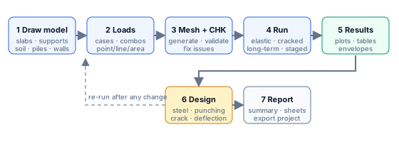
- New project → name and folder. The design code's standard load cases
(SW/SDL/LL) and combinations are created automatically. - Settings → Design - set code, f′c, fy, covers, bar, limits. These stamp
onto the model'sdesign_paramswhen you apply. - Materials - pick grades from the Material Library, or define custom
grades (project or global scope). - Draw the slab regions at their real elevations.
- Place openings, drop panels, steps (vertical plates).
- Place supports: columns, point supports, piles, walls, edge beams.
- Draw a soil zone for mats.
- Define loads: cases, combinations, then point/line/area loads and wall
top loads; switch on Self Wt where appropriate. - Draw design strips over the column and middle strips, or let the program
propose centre strips and add them. - MESH → CHK → fix anything the validator and mesh checker report.
- Run Analysis for the cases/combinations you need; read the summary.
- Inspect results - deflection, moments, bearing, reactions - and sanity
check equilibrium. - Design: required-steel maps, strip sizing, punching, crack width.
- Report: punching summary/report, charts, PDF/print; export the project.
Steps 2–3 and 9 can be revisited at any time; any geometry change marks the
solved results stale until you re-run.
1.8 Conventions in this manual
- Bold marks a UI control by its exact label.
Code fontmarks a value, field name, key or message text.- Field tables give: label, unit, default, valid range, and behaviour.
- Worked numbers in examples come from the built-in verification library and
can be reproduced with the models in
Chapter 8. - "Not implemented" boxes state the current limits honestly so you do not
look for a feature that is not there.
1.9 Current limitations
Know these before relying on the program:
Analysis scope
- Linear-elastic statics only - no modal, dynamic, buckling or thermal
analysis. - Soil springs act in tension too unless the zone is Compression only, in
which case the solver iterates uplift gaps automatically. Pile contact stays
two-way. Keep the resultant within the mat footprint unless gaps are
modelled (see §7.1). - Walls and line supports accept vertical springs only (Kz); no horizontal
soil pressure. - No moment redistribution, no second-order effects.
Modelling
- Openings must be axis-aligned rectangles fully inside one slab.
- Column stubs are meshed straight; inclined columns are not supported.
- Slabs must be flat polygons in plan; each slab has one thickness (steps are
modelled with vertical plates). - There is no undo/redo, copy/paste or mirror for loads or geometry.
- The floor plan is meshed with quads by default; triangles are available but
thinner for the same node budget.
UI
- The Clear All buttons in the slab load dialogs remove that load type for
the whole model, not just the current case. - The
After analysis showpreference is currently overridden by a hard
switch to the deflection view after a slab run. - The DXF endpoint exports the legacy frame model only (empty for slab
projects); see §9.5.
1.10 Verifying the program itself
Every formula and solver feature is benchmarked against closed-form solutions.
- Verification publishes the tables, the error of every
benchmark, and how to re-run them from the terminal. The 13 benchmark
models also ship as JSON project files inweb/projects/verification/;
import one with Import from File, run the analysis and compare against
the published values. (A dedicated verification page is planned.)
If a result disagrees with an independent hand calculation, reproduce the
nearest verification model first; if it matches there, the difference is in the
model rather than the solver.
→ Next: Chapter 2 - Modelling